Built environment heat initialization
This section describes how heating supply and demand in the built environment is initialized for the start year in the ETM. This also explains how the starting technology split is calculated by the model.
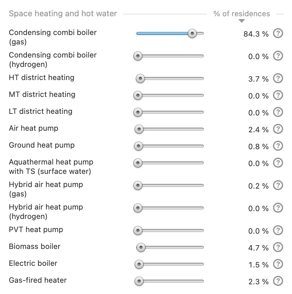
When opening a new scenario, the technology split shown in the front-end is only that of space heating technologies. The technology split for hot water technologies is not shown and may actually be different in the start year. If the slider settings are changed, both the technology split for space heating and hot water are set equally for the future year.
Overview
Supply and demand is initialized for three types of heating in the built environment:
- Buildings space heating
- Households space heating
- Households hot water
For each of these types, the generic initialization method is the same. The generic method is explained here. For the specific implementation of each type, see Heat in the built environment.
Generic initialization method
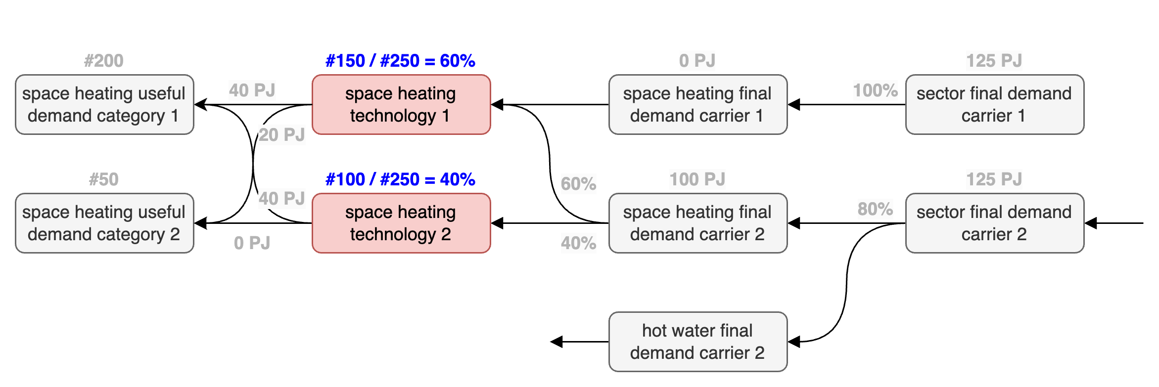
This Figure shows the generic graph design for heating in the built environment and is used to highlight the different steps in the initialization method.

There are four relevant node types for heating in the built environment. First, the final demand per carrier on a sector level. Second, the final demand per application, like space heating or hot water. Third, the heating technologies. Fourth, the useful demand nodes.
Initializing supply per technology
First, the final demand per carrier on a sector level (the yellow node) is read from the dataset of the simulated region, using the graph_methods attribute demand. Then, the split to each application (the share from the yellow node to the orange node) is determined, using the graph_methods attribute parent_share. The technology split (the share from the orange node to the red node) is then determined using parent_share as well.

This gives the total demand of the heating technology node. By taking the attribute output.useable_heat (determined in the node source analysis) as the efficiency, the supply of useable heat can be calculated.
Initializing demand per category
From the previous step, the total supply of useable heat per application per sector is known. This is equal to the total demand for useable heat. Each useful demand node (the blue node) has the attribute fever.present_share_in_demand, which can be read from the dataset using the AREA query.
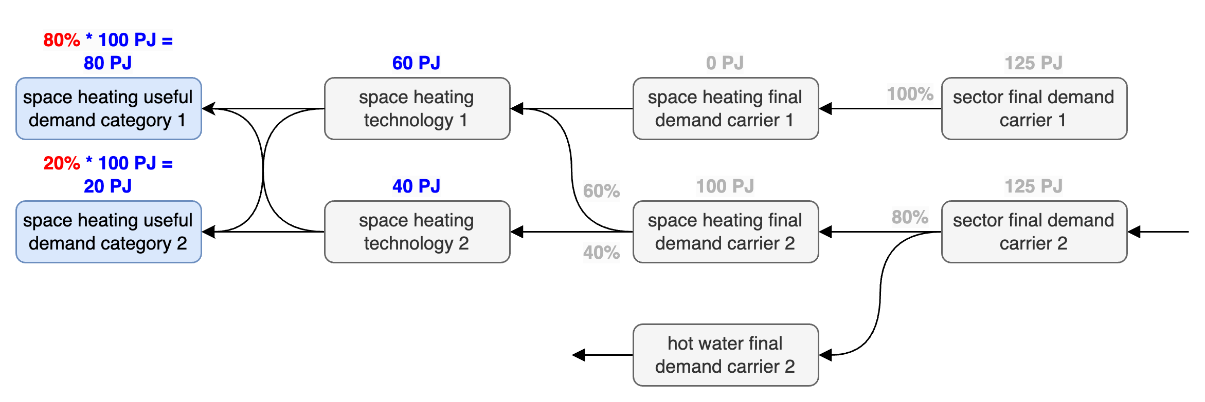
Together with the total demand, this share is used to calculate the demand for useable heat for useful demand node.
Matching supply and demand
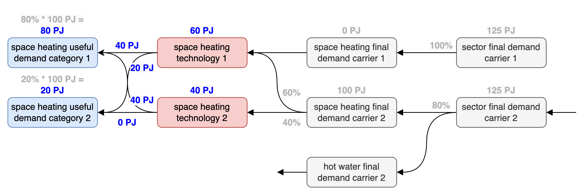
Only the edges between the heating technologies and the useful demand nodes remain to be determined. This is done using a matching algorithm and two merit orders. First, there is a supply merit order, which ranks heating technologies. Second, there is a demand merit order, which ranks useful demand nodes.
- space_heating_useful_demand_category_2
- space_heating_useful_demand_category_1
- space_heating_technology_1
- space_heating_technology_2
The first heating technology supplies the first useful demand node. If the demand is met, it moves on to the second useful demand node in the demand merit order. If its supply runs out, the second heating technology in the supply merit order starts supplying. When all demand is met, the matching algorithm is completed and the useable heat delivered on each edge is known.
Determining the technology split
For each useful demand node, the number_of_units is read from the dataset using the AREA query. For each heating technology, the share of its supply of useable heat in the input of each useful demand node is multiplied with the corresponding number_of_units. This leads to a total number_of_units for each heating technology. The sum of heating technology units equals the sum of useful demand units.
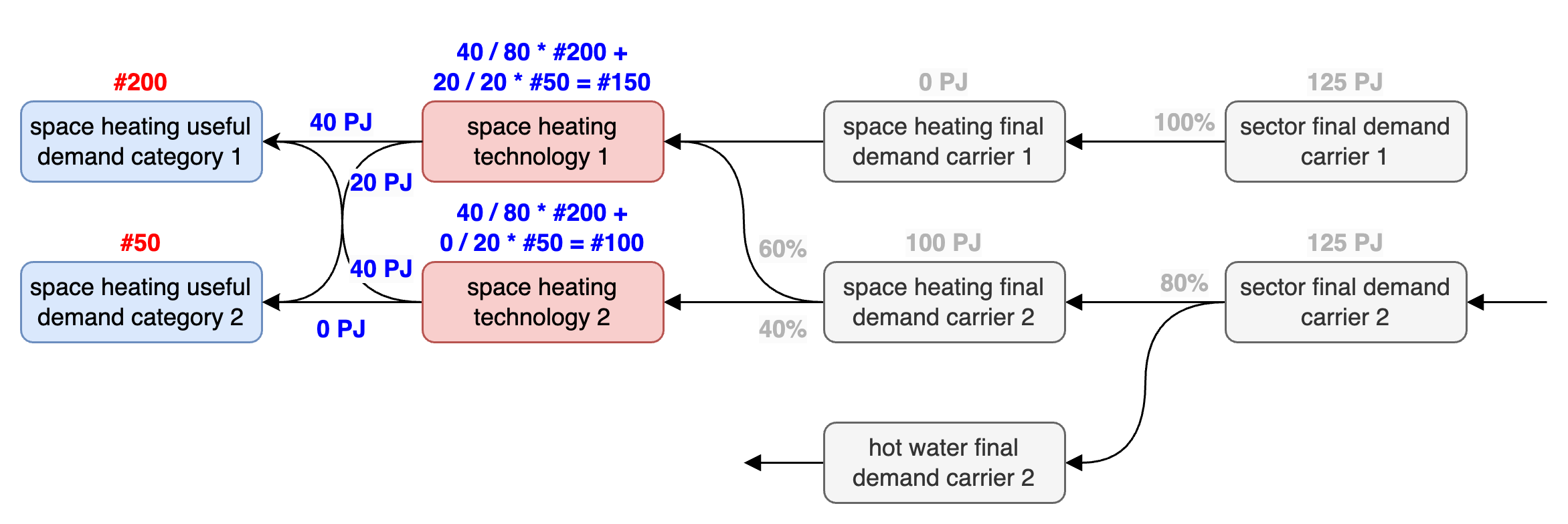
Using the share of the number_of_units each heating technology in the total, the technology split can be calculated for each sector.
