Curves
The ETM uses hourly curves to model (electricity, hydrogen and gas) demand and supply. The hourly demand and supply is determined using the annual demand and supply and a given curve. It is also possible to use your own curves in the ETM by inserting them in Modify profiles. This page gives an overview of the type of curves and explains how to modify these curves by inserting your own.
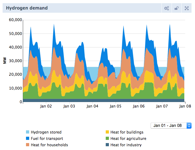
Image: Example of hourly demand - hydrogen demand
Overview of curves
The ETM had three types of curves: demand curves, supply curves and time curves. The tables below show a brief overview of the sources and methods currently used.
Demand
| Sector | Sub-sector | Source | Method | Comment |
|---|---|---|---|---|
| Households | Space heating | TNO | TNO curves fitted to temperature and irradiance which enables to generate curves for all years. Curves have been smoothed to show the average load of a cluster of 300 houses rather than an individual house. This results in lower and more realistic total demand peaks. | Update with TNO heat loss calculation when data becomes available |
| Hot water | Jordan (2001) | Distribution function based on average Dutch household. Curves have been smoothed to show the average load of a cluster of 1000 houses rather than an individual house, see GitHub | - | |
| Cooling | NEDU | E1A curve | Argumentation of method, update with TNO heat loss calculation when data becomes available | |
| Appliances, lighting, cooking | NEDU | E1A curve | - | |
| Buildings | Space heating | NEDU | G2A | Update with TNO heat loss calculation when data becomes available |
| Cooling | NEDU | E3A curve | Argumentation of method, update with TNO heat loss calculation when data becomes available | |
| Appliances | NEDU | E3A curve | - | |
| Transport | Electric cars | Movares and ELaad | Profiles available: Movares: week and weekend days for 1) charging everywhere 2) charging at home 3) fast charging. ELaad: repeating average day for 4) smart charging 5) regular charging Default curve for cars is charging everywhere. | - |
| Passenger trains, trams/metro, electric bicycle, motorcycles | Movares | 1) Charging everywhere | Aim to update with measured data (Pro Rail) | |
| Electric busses, electric trucks, freight trains | Movares | 2) Charging at home (curve peaks during night) | Update when specific data becomes available | |
| Hydrogen trucks, hydrogen busses, hydrogen cars | - | Flat curve | - | |
| Industry | Heating demand in Food, Paper and Other | Gasterra | G2C profile | - |
| Electricity demand in Food, Paper, Other and ICT | NEDU | E3D curve | - | |
| Heating and electricity in all other sectors | - | Flat curve | ||
| Agriculture | Electricity | NEDU | E3A curve | - |
| Heat | NEDU | G2A | Update when specific data becomes available |
Supply
| Sector | Source | Method |
|---|---|---|
| Solar PV | "Open Power System Data platform" | Profile from measured data, adjusted to match country specific full load hours |
| Solar Thermal | "KNMI" | Profile from measured data, adjusted to solar-thermal behaviour |
| Wind | "Open Power System Data platform" and Renewables.ninja | OPSD: Profile from measured data, adjusted to match country specific full load hours. Renewables.ninja: Modelled profiles available from 1980-present using satellite weather data. |
| Other | Geothermal heat, geothermal power, hydro, biogas CHP, waste incinerator | Flat curve |
| Dispatchable technologies | Production determined by merit order |
Time curves
Time curves define how the national production of energy carriers changes over the years (up to 2040)
They are documented in on ETDataset in the source analyses of the specific datasets. Example for the Netherlands - 2015
For the Netherlands the time curves are based on:
- Natural Gas: this GasUnie letter (31-01-2019).
- Crude oil: NLOG.
- Other carriers: The Primes reference scenario in EC 2016 Trends to 2050 - Reference Scenario 2016.
For all other countries the time curves are based on the Primes reference scenario 2016.
Checkout: the ETDataset - curves as it contains all raw data, scripts and further explanations.
Modifying Profiles
The ETM calculates the supply and demand of gas, electricity, heat and hydrogen on an hourly basis, for which it uses default curves. These curves can be modified by uploading custom curves in the Modify profiles section. Note that uploaded curves are scenario inputs; based on these profiles, the model calculates the resulting (hourly) flows.
Types of profiles
The following profile types can be uploaded:
Regular profiles. These profiles are typically used for demand profiles and represent the fraction of annual demand used in each hour of the year (8760 hours) for a specific category. The unit used in the uploaded curve file does not matter: the model uses the shape of the profile (the relative distribution of demand over time). For example, if the profile sums up to 500 and the first hour has a value of 5, 1% of the annual demand for this category is assigned to the first hour. Examples of regular profiles are: electric buses, industry heating.
Capacity profiles. These profiles are typically used for supply profiles and represent the fraction of installed capacity used for each hour of the year for a specific production technology. For example, a value of 0.5 means that 50% of peak capacity is utilised in that hour. The sum of all hours should equal the total annual full load hours of that technology. Examples of profiles are: solar PV, wind offshore. Note that a capacity profile is also used for the must-run interconnectors import and export profiles.
Price curves. These profiles are used for the interconnector prices and represent the price for each hour of the year. The unit is €/MWh and the value for each hour will be rounded to the nearest whole cent. Example profile: interconnector 1 electricity price.
Availability curves. These profiles are used for interconnector import and export availability and represent the availability of the interconnector for each hour of the year. Values should be specified between 0 and 1 for each hour, where for example 0.5 means that 50% of the capacity is available, 0 that no capacity is available or 1 that all capacity is available. Example profile: interconnector 1 import availability.
Temperature curve. Used to set the air temperature profile and represents the outdoor air temperature for each hour of the year. The unit is degrees Celsius.
Uploading a custom profile
In the curve upload section, simply choose a profile by clicking on the drop-down menu and select the specific profile to be overwritten. Click on 'Upload a custom curve' to provide a CSV file.
The CSV file should contain 8,760 rows (one for each hour per year) each with a numeric value. See additional value requirements per profile type described above.
23.64
32.71
32.65
32.71
30.89
etc
It is also possible to download the uploaded profiles in the same section. For all profile types except regular profiles, downloaded profiles are obtained in the same format as they were uploaded. When downloading a profile of type 'regular profile', a normalised profile is obtained where the shape of the orginially uploaded profile is maintained.
Results
Based on uploaded supply and demand profiles and on annual flows, the model calculates resulting hourly profiles representing the hourly energy flows. The chart on the right in the ETM section shows for all modifiable supply and demand categories the resulting hourly profiles. This means, for example, that if a capacity profile for wind offshore is uploaded, the profile depicted in the chart is not the capacity profile that represents the fraction of installed capacity deployed per hour. Instead, it shows the resulting deployed capacity in MW for each hour of the year. These resulting hourly supply and demand profiles can be downloaded in the Data export section.
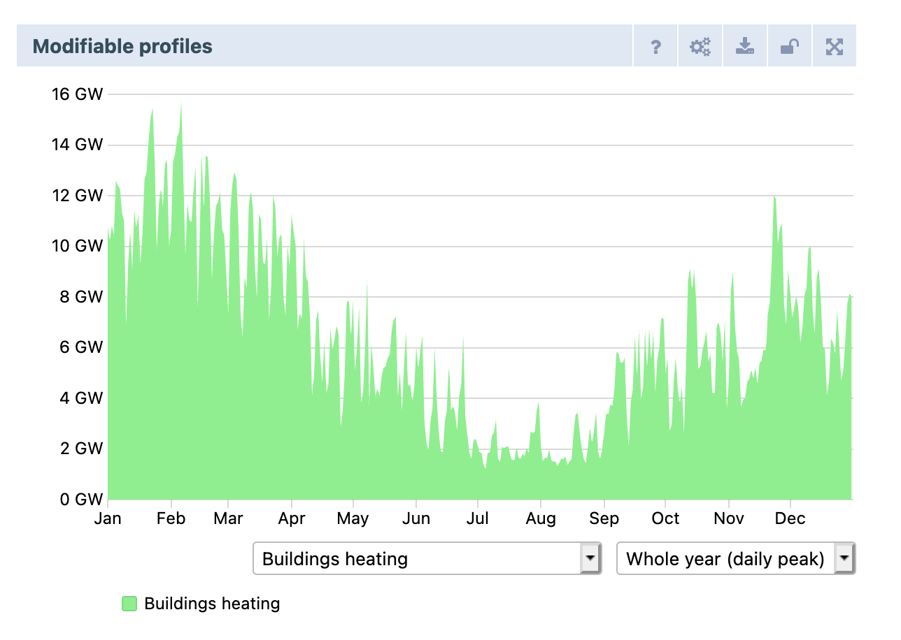
Note that if a technology is not present in the scenario, the chart series will remain empty. By default, the chart shows the daily peak capacity of the profile for the whole year. Select a month or week in the dropdown menu to see the hourly values.
Interaction with Weather Years
The ETM allows users to select different weather years. This affects all supply and demand profiles that are weather-dependent, such as heat demand and production of wind and solar power. When uploading a custom profile using the CSV upload form, the ETM always prioritises the uploaded curve over any standard curves used within the ETM. This means that even if a different weather year is chosen, any uploaded profiles will remain unchanged while other profiles will change according to that weather year.
Comments on selected profiles
The table below provides some additional information on selected categories.
| Profile | Comment |
|---|---|
| Demand: Buildings | Includes all gas, hydrogen, district heating and electricity use for heating. |
| Demand: Industry heat | Includes all gas, hydrogen and electricity use for heating |
| Demand: Industry electricity | Includes electricity demand, except electricity used for heating (boilers, heat pumps etc.) |
| Demand: Electric cars | You can upload 5 different profiles for electric cars. The ETM uses a mix of these profiles depending on your choices in the Demand response - electric vehicles section. |
| Import/Export: Gases | The ETM uses 'demand' type profiles for both import and export (see above). This means that the units used in your custom profile do not matter. The ETM will extract the shape of your profile and apply that to the annual import/export volume. |
| Import/Export: Interconnectors | See imported electricity |