District heating

In the Supply > 'District heating' section in the ETM you can specify the heat sources, transport losses and storage for district heating. If you want to know more about the modelling principles behind the use of district heating within the ETM, you can find more information below.

District heating networks

The demand, supply and storage of heat for district heating networks in households, buildings and agriculture is calculated on an hourly basis. The ETM contains heat networks for three temperature levels: LT (40 ^oC), MT (65 ^oC) and HT (90 ^oC).

Demand

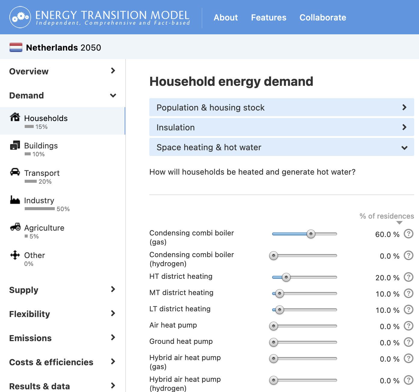
In the households, buildings and agriculture section of the model, you can make assumptions about the share of heat demand that will be supplied by district heating networks in the future. For example, in the scenario below, a total of 40% of residences is assumed to be connected to on of the three district heating networks.

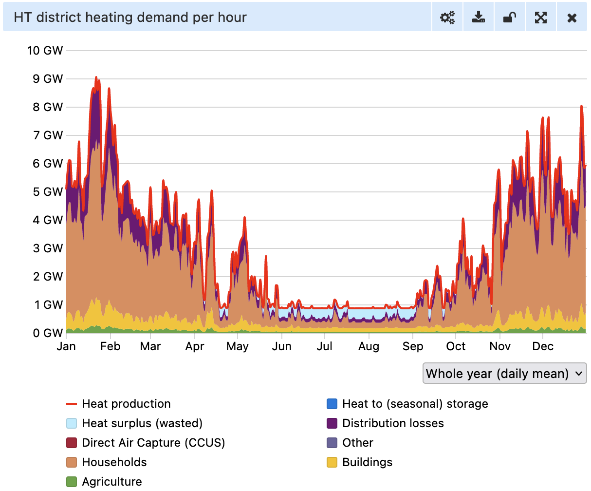
The resulting district heating demands from households, buildings and agriculture are aggregated and together make up the demand of heat networks. For each sector demand is multiplied with an hourly demand curve to estimate collective heat demand for each hour per year. More information about these curves can be found here.

Supply

You can set the installed capacities of various heating sources in the 'Supply' tab. The ETM distinguishes between two types of heat sources:

• 'Must-run' sources
• Dispatchable sources

Must-run

'Must-run' sources include all heat sources that supply heat according to a pre-defined production curve, regardless of whether there is heat demand at that moment. For example, solar thermal farms produce heat when the sun is out even if there is no demand for that heat at that moment. The ETM models the following must-run sources:

• Solar thermal
• Geothermal. We assume that geothermal heat wells produce a constant flow of heat throughout the year.
• Residual heat from the industry sector. We assume that this heat has a flat (constant) production profile.
• Imported heat from outside the region. We assume that this heat has a flat (constant) production profile.
• All CHPs:
• For biogas CHPs we assume a constant production.
• For all other CHPs we assume that their production is determined by the 'merit order' of the electricity market. If the electricity price in a given hour is high enough, CHPs will be switched on. This means that heat is a 'by-product' and that heat production is not necessarily aligned with heat demand. See documentation about the electricity merit order

Since the heat production of must-run heat sources in a given hour does not react to heat demand in that hour, it is possible that during some moments more heat is produced than is needed. It is assumed that this heat is dumped or, if heat storage is enabled, stored for later use.

Dispatchable

Dispatchable heat sources include all heat sources that can be turned on and off at will. Their production profiles are determined dynamically: in a given hour, dispatchable heat sources will only produce heat if the demand in that hour exceeds supply of must-run sources. Dispatchables will switch on to ensure that supply matches demand. The ETM models the following dispatchable heat sources:

• Gas and hydrogen burners
• Electric heat pumps
• Biomass and waste heaters
• Oil, coal and lignite heaters
• Aquathermal heaters
• Heat storage. See the Storage section below.
• A back-up/emergency heater using network gas

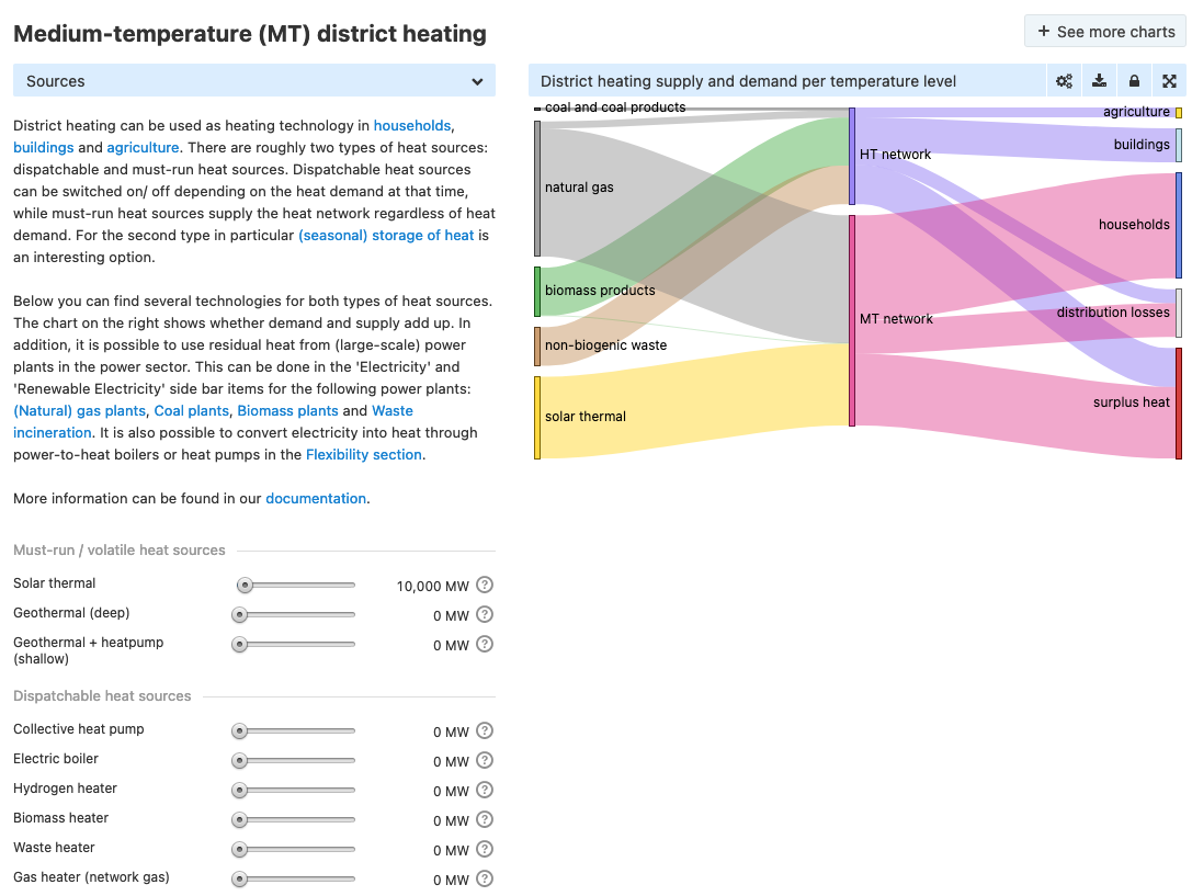
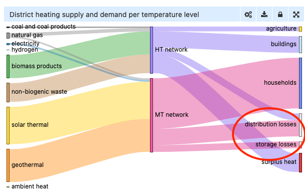
For each of these heaters you can set the installed capacity in the 'District Heating' section of the ETM. The only exception to this is the back-up heater. The ETM automatically determines the required amount of gas burner back-up capacity to ensure that supply always meet demand in every hour. This will show up as natural gas in the 'District heating supply and demand per temperature level' chart (see below for an example where for the MT heat network just 'Solar thermal' is set). You can decrease this shortage by increasing the installed capacity of other dispatchables.

Merit Order

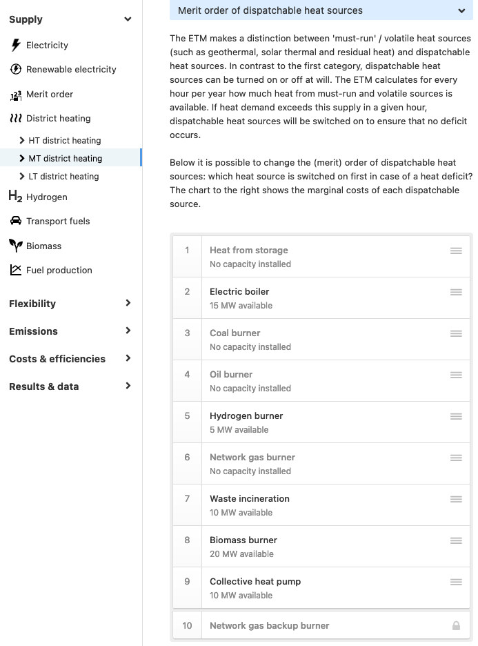
When multiple dispatchable sources are installed, a heat 'merit order' determines which dispatchable switches on first. The back-up burner always comes last ('lender of last resort'). By default, the merit order is based on marginal production costs. This can be changed in the Merit Order subsection of District Heating.

Example: Suppose that in hour X heat demand is 100 MW and that must-run sources supply 20 MW. This means that 80 MW will be supplied by dispatchables. Now suppose that you install 30 MW of biomass heaters, 50 MW of heat pumps and 20 MW of gas heaters and that you alter the heat merit order such that biomass comes first, followed by heat pumps and gas heaters. Since biomass is first in line, the heater will turn on in hour X, supplying 30 MW of the 80 MW residual demand. This leaves a residual demand of 50 MW. Thus, the heat pumps switch on as they are second in line, supplying 50 MW. The gas heaters will not switch on in this hour as heat demand has been fully met.

Heat storage

As seen above, must-run heat sources supply heat regardless of heat demand. As such, it is possible that heat is produced during hours of low or no heat demand. This heat is registered as a 'heat surplus'. One striking example is solar thermal farms, which produce a lot of heat during summer when heat demand is low.

To avoid large amounts of dumped heat you can decided to use (seasonal) heat storage. This can be done by switching the storage toggle to 'On'.

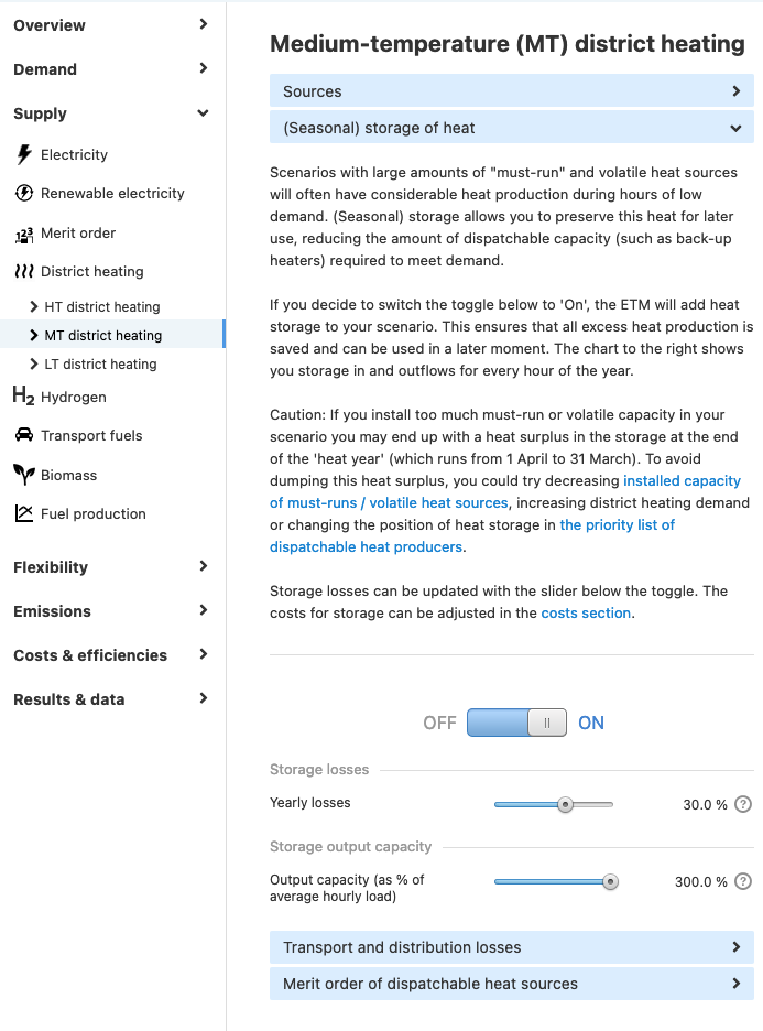
When switched on, the ETM automatically installs sufficient storage volume to store all heat surpluses of must-run producers. This heat can be used later on in the year, allowing for a more efficient use of must-run capacity and a lower need for dispatchables.

Storage as dispatchable

Heat storage is considered a dispatchable heat source. This means that heat will be drawn from storage during moments that heat demand exceeds must-run supply. By default, heat storage comes first in the heat merit order, which means that in case of a shortage in supply, heat is drawn from storage before other dispatchables (like gas burners) are switched on. Of course it is only possible to draw heat from storage if this heat has been put into storage earlier on in the year. You can change the merit order positions in the Merit order subsection. Moving heat storage to a lower position in the merit order results in a slower depletion of stored heat. See Merit order.

The output capacity of heat storage is unlimited by default. This means that there is no limit to the amount of heat that can be drawn from storage in one hour (given that enough heat is available in the storage). You can limit this with a slider. A lower output capacity can result in a slower depletion of heat storage. A consequence of this could be that other dispatchable heat sources (such as gas heaters) need to be switched on earlier: if the output capacity of storage is insufficient to meet demand in a given hour, other dispatchables need to be switched to guarantee that enough heat is supplied.

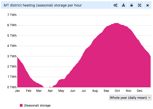
The 'heat year'

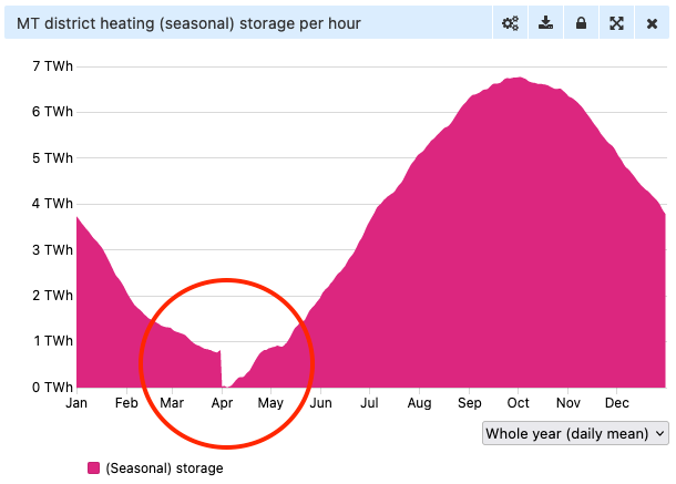
At the start of the 'heat year', storage is assumed to be empty and is subsequently filled over time when heat surpluses arise. Since heat demand is typically concentrated in winter, it is undesirable to start with an empty storage on 1 January. Therefore, the hourly calculation starts on 1 April and runs until 31 March. On 31 March, any excess heat that remains in the storage is 'dumped' to ensure that every year the same amount of heat is drawn from storage as is put into it.

If this 'dumping' of excess heat in storage is significant, a 'hick-up' can be seen in the hourly storage chart (see below). This hick-up can be resolved by decreasing the installed capacity of must-run sources, by increasing demand for district heating or by moving heat storage up in the heat merit order.

Storage losses

Heat storage is subject to thermal losses. You can set a yearly loss percentage with a slider. This percentage is converted to a loss percentage per hour ((yearly losses)^(1/8760)). For every hour per year this hourly percentage is multiplied with the heat in storage at that moment to calculate storage losses in that hour.

This means that the total storage losses are typically (much) lower than the yearly loss percentage set by you. If 100 TJ heat is stored and yearly losses are 20%, it is generally not the case that 20 TJ heat is lost. Only if heat storage is filled on day 1 and no heat is drawn from storage during the year, the total heat lost is equal to the yearly loss percentage. In practice the storage is filled over a longer period of time and also emptied over time, which means that heat is typically stored for a shorter period than a full year, resulting in lower losses.

Transport and distribution losses

District heating networks have significant heat losses. In the ETM this is taken into account by proportionally increasing demand for each hour per year.

Loss is expressed as a percentage of total supply. This percentage can be changed by you with a slider. For modern district heating networks a loss of 15-20% is common. For older networks, heat losses can range from 30%-40% or even higher.

Please note that the default loss value for many regions in the ETM is either fairly low or even zero. For countries, losses are determined based on data from the energy balance of the International Energy Agency. In The Netherlands, for example, only a small percentage of houses and buildings is currently connected to a district heating network whereas relatively many agricultural buildings are, mainly in the greenhouse industry. These greenhouses are typically located close to each other, with most of the heat sources (CHPs) on-site. This results in low average losses of all district heating networks combined.

For other regions in the ETM, such as municipalities or neighbourhoods, there is typically no reliable data source on heat distribution losses, resulting in a zero default value.

If district heating in the built environment plays a significant role in your scenario, it is advised to change the distribution losses to the percentages recommended above.

The annual distribution and storage losses are shown in the chart 'District heating supply and demand per temperature level'.

Infrastructure costs

Checkout: the 'Heat infrastructure costs' infopage for more information.

Industrial heat network

Heat networks in the industry sector are modelled in a much simpler fashion. Supply and demand are calculated on a yearly basis. You can set the heat demand for each industry sub sector and can select the heat sources in the 'Heat network sources' tab.

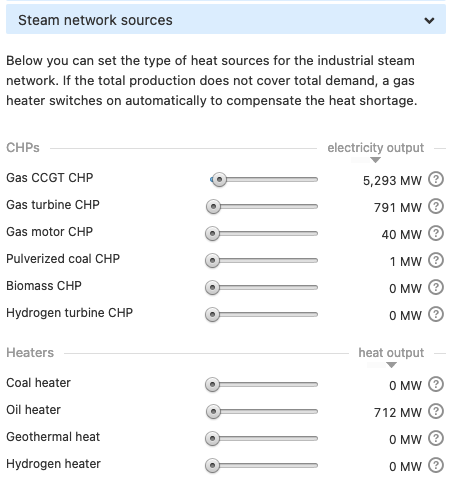
For heaters and geothermal, total production per year equals installed capacity times a fixed number of full load hours. More information can be found when clicking the '?' icon next to a heat source and opening that 'Technical and financial properties' table.

For CHPs, full load hours are scenario dependent: they are determined by the electricity merit order. Industry CHPs will produce whenever the electricity price is lower than their marginal production costs. For more information, see the CHP section in the merit order documentation for more information.